> For the complete documentation index, see [llms.txt](https://help.multiomics.illumina.com/llms.txt). Markdown versions of documentation pages are available by appending `.md` to page URLs; this page is available as [Markdown](https://help.multiomics.illumina.com/icm/analyses/analysis-functionality/data-viewer/chromosome-view/customizing-the-view.md).
# Customizing the View
## Controls
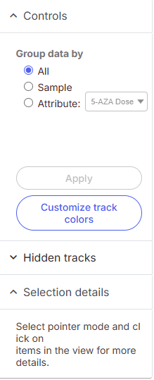
*Chromosome view* can be customized by using the control panel on the left. The *Group data by* option specifies the number of *Alignments* tracks. The *Attribute* and *Order by* controls show options depending on the current analysis. In order for any change to take place, push the **Apply** button.
#### **All**
*All* will result in only one track, with all the samples on it.
#### **Sample**
*Sample* creates one track per sample, with option to *Order by* sample attribute.
#### **Attribute**
*Attribute* produces one *Alignments* track per level of the *Attribute* (i.e. one track per group).
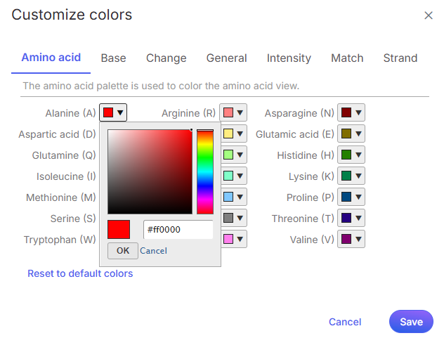
#### Customize track colors
To change any of the colors on the canvas, use the *Customize track colors* tool. A resulting dialog will help you to pick another color (**drop-down** button opens the color-picker).
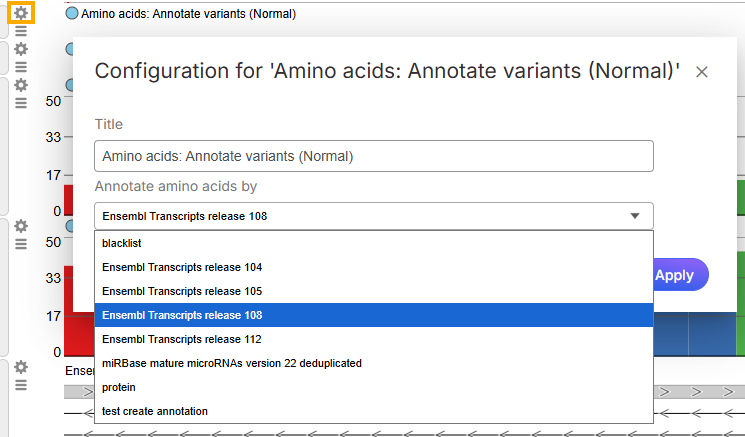
## Annotate amino acids by
*Annotate amino acids by* option controls the appearance of the *Amino acids* track and allows you to pick the transcript database that will be used to plot codons. It can be customized by clicking setting  icon on *Amino acids* track. In the *Configuration* dialog, select an annotation file from the *Annotate amino acids by* drop down list. The drop down list shows annotation files associated with the current genome build.
## Color by
*Color by* option affects the colouring of the *Alignments* track and *Isoform proportion* track. It can be customized by clicking setting  icon on aforementioned tracks. In the *Configuration* dialog, *Sample*, *Base*, and *Match* options are present by default, if attributes have been assigned to samples, they will appear in the drop-down list. In figure below, that are the "Type" and "Subject ID" attributes.
#### Color by Sample
When *Sample* is selected from the *Color by* drop-down list, individual samples will be shown on the track, each sample being given a different colour.
#### Color by a sample attribute
When a sample attribute is selected from the *Color by* drop-down list, different colors will be used to depict levels of the selected sample attribute (as present in the Metadata tab).
#### Color by Base
The effect of the option to *Color by Base* can be seen with high power magnification. Individual base calls are highlighted by different colours. When that option is chosen at low power magnification, all the bases are shown in grey.
#### Color by Match
*Color by Match* option can be used to quickly identify mismatches against the reference genome. A matching base is coloured in blue, while mismatch bases are colored in yellow.
## Histogram type
*Histogram type* changes the presentation of the *Alignments* track. It is customizable on *Configuration* dialog invoked on the *Alignment* track, and should be used in conjunction with the *Group data by* and *Color by* tracks to get the desired visualisation.
When set to *Sum*, the *histogram type* shows the sum of base calls at each position, i.e. total coverage per position. Figure below shows an *Alignments* track with three samples. With the *Sum* option, the number of reads at each base in each sample is added and displayed. The contribution of individual samples is not visible since the track is *Colored by Group* (but that would make sense in this example).
To show the average coverage per locus, switch *histogram type* to *Average* and leave *Color by* as is (i.e. by group). With this setting, *Chromosome view* will calculate the average by dividing the total coverage per locus by the number of samples. Note that using *Color by Sample* would not make sense here. Note the difference in y-axis range in figure below compare to the figure when the *histogram type* was set to *Sum*.
Finally, the option *Overlay* is useful if you want to directly compare base counts over several samples (or groups) as each will be represented by a line (i.e. no stacking). The example in figure below is based on microarray data, showing three groups on the same *Alignments* track. The red group has the highest base counts, while the counts in the blue group are much lower.
## Y-axis max
The maximum of the y-axis of *Alignments* tracks is set by *Y axis max* option in *Configuration* dialog invoked from the *Alignments* track. When using *Project max*, all the tracks have the same Y axis maximum, which depends on the sample with the highest coverage. On the other hand, *Track max* uses independent Y axis maximum for each track.
#### Project max
#### Track max
## Split by strand
To view the histogram grouped by the specific strand that they've mapped to, click the *Split by strand* checkbox in the *Configuration* dialog on *Alignement* track. This displays the forward reads at the top half of the track and the reverse reads on the bottom half of the track. This track can be helpful in studies such as ChIP-Seq, where strand-specific read distributions can display hallmarks of DNA-protein interactions.
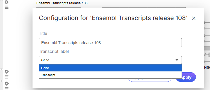
## Transcript label
You can use the *Transcript label* option to specify labels on the reference transcript track and *Isoform proportion* track. Click *setting*  icon on aforementioned tracks to open the *Configuration* dialog. Both transcript database and Isoform proportion tracks of Short sequencing reads can be coloured by strand (Reads pileup color: Strand) or by base (Reads pileup color: Base).
#### Transcript label: Gene
#### Transcript label: Transcript
## Reads pileup and probe color
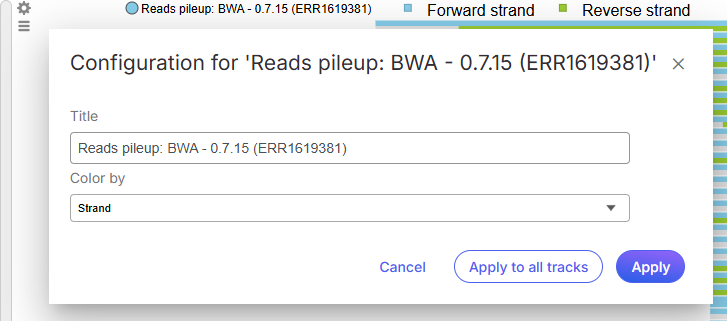
*Reads pileup* track can be displayed on *Chromosome View* by selecting Short Sequencng Reads data from *Select tracks* tool. Click *setting*  icon on the *Reads pileup* track to open *Configuration* dialog, two options are available to color the reads pileup: *strand*, *base*.
#### Reads pileup color: Strand

#### Reads pileup color: Base

*Probe color* control customizes the appearance of *Probe intensities* track. When set to *Intensity*, the color of a probe reflects its intensity, using a color gradient from white (low) to admiral (high). Alternatively, when *Strand* is turned on, probes on the reverse strand are in parakeet green, while probe on the forward strand is in sky blue.
#### Probe color: Intensity
#### Probe color: Strand
## Variant database
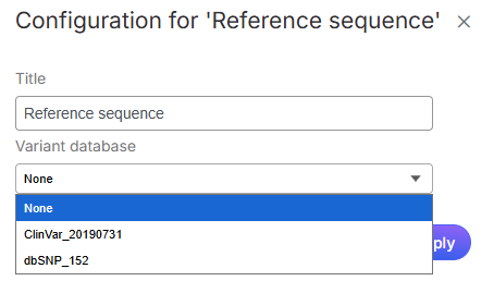
If a variant database is available for the current genome, the variants can be added to the [*Reference genome* track](/icm/analyses/analysis-functionality/data-viewer/chromosome-view/annotating-the-results.md#reference-genome). To show the variants, point the *Variant database* control to the database of your choice.
## Track Order
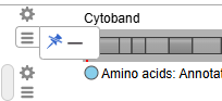
The position of the tracks on canvas can be controlled by using the *Track order*  tool on the left of each track. If you want a track to be visible all the time, i.e. while scrolling up or down, pin it to the top or to the bottom. Below shows the *Cytoband* track pinnned to the top of the canvas. To unpin a track, click on the **pin icon** .
To pin a track, click the green arrows to pin a track to the top or bottom of the view. When you mouse over an arrow, the new position of the track will be highlighted on the canvas; click on the **arrow** to accept.
A track can be hidden (meaning it will not be visible) by selecting the **minus icon.**
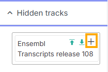
Hidden tracks can be unhidden by selecting the **plus** icon at *Hidden tracks* section on the left panel.
The tracks can be reordered by **drag and drop**.
## Selection Details
At the bottom of the control panel you will find the *Selection details* section. It is used to display information on the element selected on the canvas (using the *Pointer mode*). Example below shows details of a microarray probe. Note the two link-outs ("Browse on UCSC" and "BLAST this sequence")
---
# Agent Instructions
This documentation is published with GitBook. GitBook is the documentation platform designed so that both humans and AI agents can read, navigate, and reason over technical content effectively. Learn more at gitbook.com.
## Querying This Documentation
If you need additional information that is not directly available in this page, you can query the documentation dynamically by asking a question.
Perform an HTTP GET request on the current page URL with the `ask` query parameter, and the optional `goal` query parameter:
```
GET https://help.multiomics.illumina.com/icm/analyses/analysis-functionality/data-viewer/chromosome-view/customizing-the-view.md?ask=&goal=
```
`ask` is the immediate question: it should be specific, self-contained, and written in natural language.
`goal` is optional and describes the broader end goal you are ultimately trying to accomplish on behalf of the user. GitBook uses it to tailor the answer towards what is most useful for that goal.
The response will contain a direct answer to the question and relevant excerpts and sources from the documentation.
Use this mechanism when the answer is not explicitly present in the current page, you need clarification or additional context, or you want to retrieve related documentation sections.
%20(1).png?alt=media)
%20(1).png?alt=media)
%20(1).png?alt=media)
.png?alt=media)
.png?alt=media)

%20(1).png?alt=media)
%20(1).png?alt=media)
%20(1).png?alt=media)
%20(1).png?alt=media)
%20(1).png?alt=media)
%20(1).png?alt=media)

%20(1).png?alt=media)
%20(1).png?alt=media)
%20(1).png?alt=media)
%20(1).png?alt=media)


%20(1).png?alt=media)